Markov Chains Simply Explained!

If you ever read data science or mathematics papers, you probably have seen or heard about Markov Chains. In this post, I will explain to you in very simple words what Markov Chains are, how they work, and why and how they can be useful.

Introduction

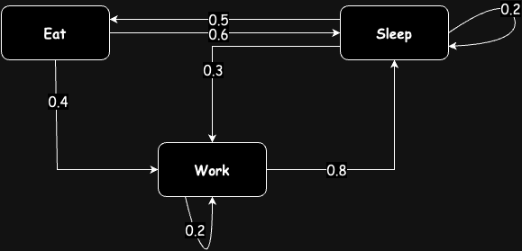
Imagine you want to model a person’s states as three states: Eating, Sleeping, and Working. This is not a realistic modeling of a person’s activities, but it’s a good example for us to understand Markov chains. Let’s assume that the initial state is ‘Sleeping’. After we sleep and wake up, there is a 0.2 probability of going back to sleep, a 0.3 probability of going to work, and a 0.5 probability of eating. The same type of probabilities exists for transitions from the other states, and you can see the probabilities for each transition from one state to another in the diagram below.

There is a very important property of Markov chains that we should always remember:

Important Property: The future state depends only on the current state, not on the previous states. ¹

Or in mathematical terms, we can describe it as:
\(P(X_{n+1} = x \mid X_n = x_n).\)

This is just the basic variation of Markov chains. There are other variations as well, but here we only discuss the basic Markov chain.

Probability of States

One common question is: “What is the probability of being in a certain state?” For example, what is the probability that a person is sleeping or working?

We can use a technique called a “random walk” to simulate the transitions between states and observe how the probabilities evolve over time. If we perform an infinite number of steps, the probabilities may converge to a stable distribution.

The probability distribution that you get after performing an infinite number of steps is called the “stationary distribution” or the “equilibrium state.”

Transition Matrix

A more efficient way to represent a Markov chain, rather than just a visual diagram, is using an adjacency matrix, also known as a transition matrix. This matrix, usually denoted as ( A ), contains the probabilities of transitioning from one state to another.

We define a row vector ( \pi ) that represents the probability distribution of being in each state:
\(\pi = [\pi_0, \pi_1, \pi_2, \ldots]\)

Each element ( \pi_i ) represents the probability of being in state ( i ).

If we multiply this initial distribution vector ( \pi_0 ) by the transition matrix ( A ), we get the distribution of probabilities after one step:
\(\pi_1 = \pi_0 A\)

If we continue this process iteratively, such that:
\(\pi_2 = \pi_1 A = \pi_0 A^2, \quad \pi_3 = \pi_2 A = \pi_0 A^3, \ldots\)

Eventually, if we reach a state where the output vector equals the input vector (i.e., ( \pi_{n+1} = \pi_n )), then we have reached the stationary state.

Mathematically, this can be expressed as:
\(\pi A = \pi\)

This equation resembles an eigenvector equation, where ( \pi ) is the eigenvector and ( A ) is the matrix. To find the stationary distribution, we solve this equation along with the condition that the sum of the probabilities must equal 1:
\(\pi_0 + \pi_1 + \ldots + \pi_n = 1\)

By solving this, we can determine the stationary state distribution for the Markov chain.

Conclusion

Markov chains provide a powerful mathematical framework for modeling systems that undergo transitions from one state to another, where the future state depends only on the current state. They are widely used in various fields, including economics, genetics, game theory, and artificial intelligence, due to their simplicity and ability to model complex stochastic processes.

Read More

1. Normalized Nerd Youtube Playlist ↩︎